
Reading Time: 10 Minutes
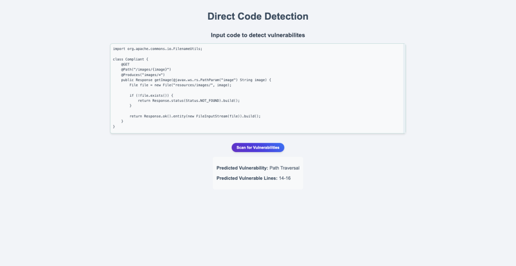
In our paper “Unleashing LLMs for High-Level Java Vulnerability Detection” Aditya Balaji, Kannan Ramamoorthy, Ejaet, Volume 12 Issue 8, 2025, 16-21 we propose a tool for High-Level Java Vulnerability detection using Large Language Models (LLMs). Our objective is to solve the shortcomings of traditional automation tools for source code vulnerability detection that have a limited scope and constrained rule sets, which may not detect certain vulnerabilities.
Our tool enables developers and testers to scan and isolate complex Java code vulnerabilities beyond the scope of automation tools. By integrating our tool as a pipeline into their platform, users can easily identify vulnerabilities.
Our research paper covers all the theoretical concepts and methodologies we have followed to build our tool, in this post we aim to break down the coding behind the tool and how we achieved our goal. We highly recommend you to read the paper once in order to understand the logical steps that we code in this post.

Coding the Tool
1. Data Collection
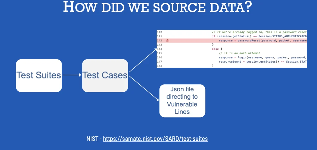
To obtain the data for training our model, we researched for various sources and found NIST test suites to be the right fit. By right fit, we mean the semantic variations in the dataset for the model to learn useful information and clarity in code.
We directly downloaded the test suites for java from the official website and preprocessed it using python’s json library to scan the required columns. The extracted data and processed data from NIST and processed using pandas and then converted into Hugging Face’s datasetdict format with this structure.
Dataset ({
features: [Vulnerability, ‘Vuln_Lines’],
num_rows: 2560
})
From an AI model training perspective this volume of data needs to be improved, but due to dataset limitations we had to work on building optimized architectures for our model and optimizing hyperparameters to give the best outcome. The below
The below code explains how we extraced the required lines and the code file to be scanned.
data = json.load(json_file)
vuln_det = {}
run = data.get("runs")[0]
for result in run.get("results"):
    message = result.get("message").get('text') #there is only one vulnerability per file
    uri = ''
    loc_list = []

    if result.get('locations'):
        for location in result.get('locations'): # there could be multiple locations
            sub_code_lines = ""

            startLine = location.get('physicalLocation').get('region').get('startLine')
            endLine = location.get('physicalLocation').get('region').get('endLine')
            uri = location.get('physicalLocation').get('artifactLocation').get('uri')
2. Data Processing
Once we had the data extracted, then we cleaned for duplicates and inconsistencies. We found that we had 62 unique vulnerabilities across various classes. Which was the effectively mapped onto 10 categories to avoid class imbalance which can distort model’s prediction abilities. This is a reference plot to visualize the class imbalance.
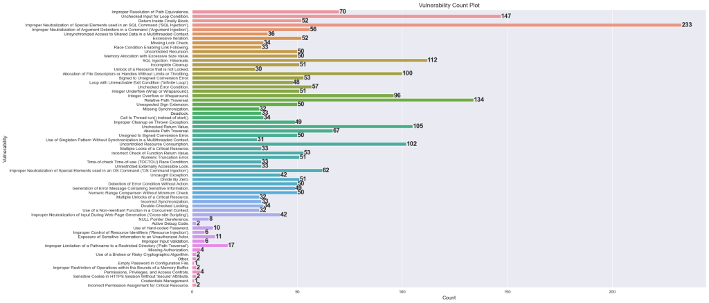
After lots of discussion for merging, we arrived at this graph ->
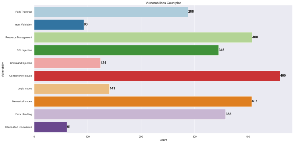
All the visualization and analysis was performed on python with seaborn and matplotlib libraries.
3. Building the Model
For this problem statement we decided to go with the (encoder only – suitable for classification tasks) basic BERT model consisting of 110 million parameters, as it allowed as to configure the fine-tuning part without any added architectural complexities.
So the first step was to get clear with the tokenization and setting max_length, for that we have explained the paper on how we accomplished the right settings. The below code explains the class we created to process the data for the model.
from transformers import AutoTokenizer
import torch

tokenizer = AutoTokenizer.from_pretrained('bert-base-uncased')

class VulnDataset(Dataset):
    def __init__(self, code, labels, tokenizer, max_length):
        self.code = code
        self.labels = labels
        self.tokenizer = tokenizer
        self.max_length = max_length

    def __len__(self): # This is required as the Dataloader for batching the data reuires a len method, not defining will lead to TypeError: object of type 'VulnDataset' has no len()
        return len(self.code)

    def __getitem__(self, idx):
        code = self.code[idx]
        label = self.labels[idx]
        encoding = self.tokenizer(code, return_tensors='pt', max_length=self.max_length, padding='max_length', truncation=True)
        return {'input_ids': encoding['input_ids'].flatten(), 'attention_mask': encoding['attention_mask'].flatten(), 'label': torch.tensor(label)}
The basic model can be loaded with BertModel.from_pretrained(‘bert-base-uncased’) (from transformers import BertModel). Since we are adding layers to predict on 10 classes, we created a class to do so.
class BERTforVulnDetection(nn.Module):
    def __init__(self, bert_modelname='bert-base-uncased', num_classes=10):
        super(BERTforVulnDetection, self).__init__()
        self.bert = BertModel.from_pretrained(bert_modelname)
        self.forward_prop = nn.Linear(self.bert.config.hidden_size, num_classes) # helps in dimentionality reduction, usually it is 768 dimensions
        self.dropout = nn.Dropout(0.3) # it helps in preventing overfitting

    def forward(self, input_ids, attention_mask):
        output = self.bert(input_ids=input_ids, attention_mask=attention_mask)
        pooled_output = output.pooler_output # fetches the hidden state corresposding to [CLS] token
        x = self.dropout(pooled_output)
        logits = self.forward_prop(x)
        return logits

# Setting the hyperparameters - this was decided after various configurations during training
bert_model_name = 'bert-base-uncased'
num_classes = 10
max_length = 140
batch_size = 8
num_epochs = 2
learning_rate = 1e-5

device = torch.device('cuda' if torch.cuda.is_available() else 'cpu')
model = BERTforVulnDetection(bert_model_name, num_classes).to(device)We trained the model on a Nvidia GPU, but this setup can be trained on CPU as well which will take a significantly longer. Instructions to setup Nvidia GPU for AI training locally can be found on my post below.
4. Preparing Data for Training
It is a general rule in AI to split dataset into train and test in order to measure the performance of the trained model.
from sklearn.model_selection import train_test_split
train_texts, val_texts, train_labels, val_label = train_test_split(dataset['vuln_lines'], dataset['labels'], test_size=0.2, random_state=42)

train_dataset = VulnDataset(train_texts, train_labels, tokenizer, max_length)
val_dataset = VulnDataset(val_texts, val_label, tokenizer, max_length)

train_dataloader = DataLoader(train_dataset, batch_size=batch_size, shuffle=True)
val_dataloader = DataLoader(val_dataset, batch_size=batch_size)
Batch training is one of the crucial concepts in AI training that helps in various aspects such as:
- Smooth updates: mitigates the possible harsh impact from any individual sample’s gradient, hence leading to more stable and consistent updates.
- Handling outliers: it helps avoid erratic parameter updates that can arise due to unremovable outlier datapoints that could play an important role in data dynamics.
- Approximation of Full-batch Gradient: allows to make meaningful progress with less data, saving on compute and time.
- Variance Reduction: makes the optimisation path less noisy and prevents vanishing/ exploding gradients.
5. Evaluation Function
This step is usually after the model training, but since we wanted to track the progress of model across n number of epochs, we defined a dedicated evaluation function.
def evaluate(model, data, device='cuda'):
    model.eval()
    predictions = []
    actual_labels = []
    with torch.no_grad():
        for batch in data:
            input_ids = batch['input_ids'].to(device)
            attention_mask = batch['attention_mask'].to(device)
            labels = batch['label'].to(device)
            outputs = model(input_ids=input_ids, attention_mask=attention_mask)
            _, preds = torch.max(outputs, dim=1)

            predictions.extend(preds.cpu().tolist())
            actual_labels.extend(labels.cpu().tolist())


return accuracy_score(actual_labels, predictions), classification_report(actual_labels, predictions)6. Training Function
Now that the evaluate function is defined, we need to prepare the train function that learns form the data and tracks the progress.
def train(model, data, optimizer, scheduler, total_steps, validation_interval, val_dataloader, device='cuda'):
    model.train()
    total_loss = 0
    losses = []
    progress_bar = tqdm(range(total_steps), desc="Training")

    data_iterator = cycle(data)

    for current_step in range(total_steps):
        element = next(data_iterator)
        optimizer.zero_grad()

        input_ids = element['input_ids'].to(device)
        attention_mask = element['attention_mask'].to(device)
        labels = element['label'].to(device)

        # Forward pass
        outputs = model(input_ids=input_ids, attention_mask=attention_mask)
        loss = nn.CrossEntropyLoss(label_smoothing=0.1)(outputs, labels)

        # Backward pass and optimization
        loss.backward()

        optimizer.step()
        scheduler.step()

        # Track loss
        total_loss += loss.item()
        losses.append(loss.item())

        # Update progress bar
        progress_bar.set_postfix(loss=loss.item())
        progress_bar.update(1)

        # Validation after every "epoch-equivalent"
        if (current_step + 1) % validation_interval == 0:
            accuracy, report = evaluate(model, val_dataloader, device)
            print(f"\nStep {current_step + 1}: Validation Accuracy: {accuracy:.4f}")
            print(report)

    progress_bar.close()
return losses, reportNow that all the functions are defined, the hyperparameters are set for optimizer and scheduler.
optimizer = torch.optim.AdamW(model.parameters(), lr=learning_rate)
total_steps = len(train_dataloader) * num_epochs
scheduler = get_linear_schedule_with_warmup(optimizer, num_warmup_steps=int(0.1 * total_steps), num_training_steps=total_steps) # warming up using 10% of the total_steps
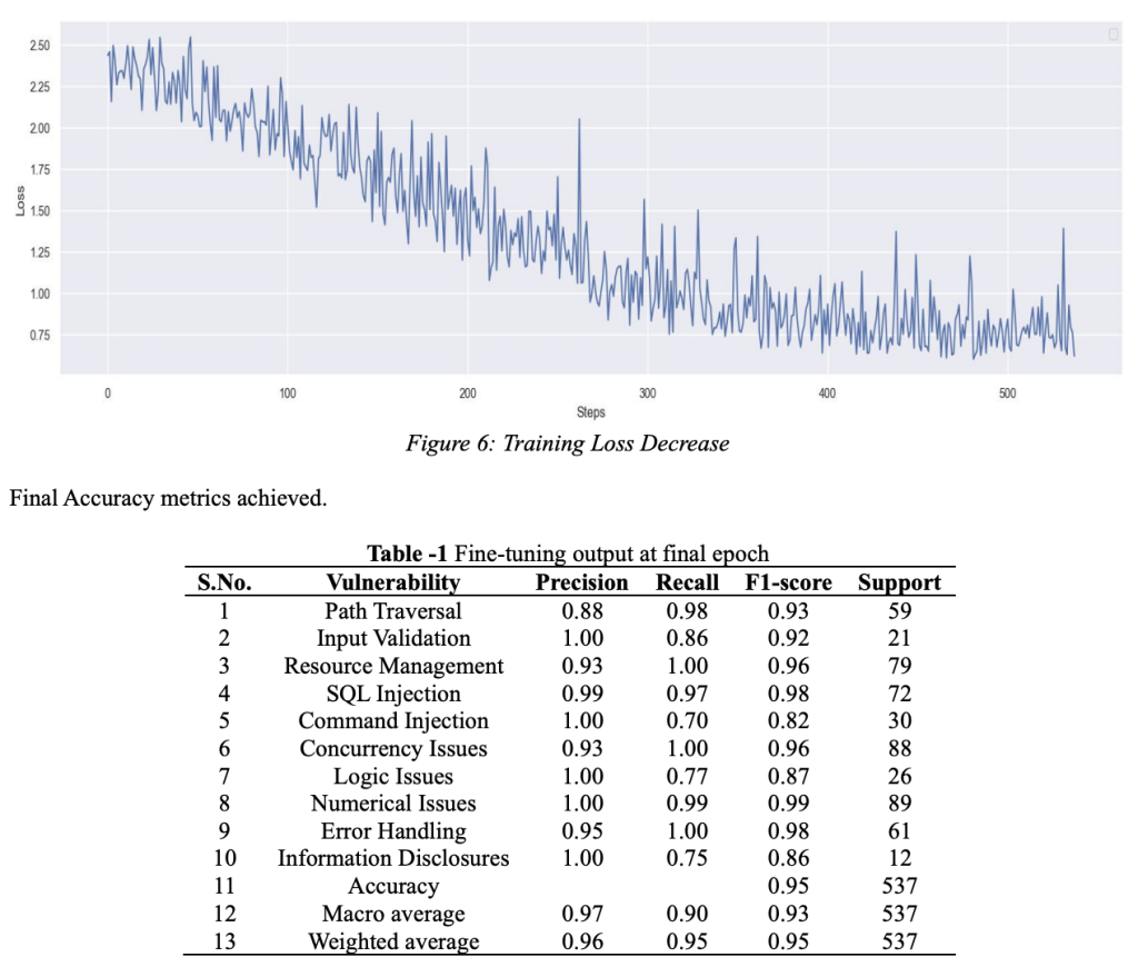
la, report = train(model, train_dataloader, optimizer, scheduler, total_steps, len(train_dataloader), val_dataloader, device)7. Negative log-likelihod
It tells us the rough area where the initial loss should be.
import numpy as np
-np.log(1/10) # = 2.30You can see that in the loss curve the initial loss is at 2.4 and decreases to 0.75. Which depicts that the model has learnt useful information in the training phase.
That’s a wrap, this post has now covered the main concepts we used to build the model, more information on pre-processing the user data at model inference can be found on our paper. Thank you for reading along, do post your thoughts and suggestions in the comment section below.
Follow and subscribe to sapiencespace for more such insights.
Link to AI and Data Science related posts: https://sapiencespace.com/data-science-programming/
Link to Cybersecurity related posts: https://sapiencespace.com/cybersecurity/
cover and title image credits: unsplash content creators


